📊 Project Overview

 A comprehensive data analysis project that demonstrates the complete data pipeline from data collection to visualization. The project analyzes sales, profit, and revenue data using various tools and technologies.

🛠️ Technologies Used

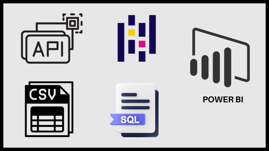
• Python (Pandas) for data cleaning
• Kaggle API for data collection
• PostgreSQL for data storage and analysis
• Power BI for visualization
• SQL for data querying

 Project Structure

1. Data Collection
2. Data Cleaning (Python/Pandas)
3. Database Operations
4. Data Analysis 
5. Data Visualization (Power BI)

📋 Project Explanation

1. Data Collection

Utilized Kaggle API to fetch CSV datasets

Automated data retrieval process

2. Data Cleaning (Python/Pandas)

Handled missing values

Standardized data formats

Created derived columns

Removed duplicates

a. Initial Setup and Data Download

# Import required library for Kaggle API import kaggle # Download CSV file from Kaggle !kaggle datasets download ankitbansal06/retail-orders -f orders.csv # Extract file from zip import zipfile zip_ref = zipfile.ZipFile(‘orders.csv.zip’) zip_ref.extractall() # extract file to current directory zip_ref.close() # close file # Read the CSV file into a pandas DataFrame import pandas as pd df = pd.read_csv(‘orders.csv’)

This section:

Uses the Kaggle API to download a retail orders dataset Extracts the downloaded zip file Loads the data into a pandas DataFrame

b. Data Exploration and Analysis

df.head() # View first few rows df.shape # Get dimensions of DataFrame df.info() # Get DataFrame information df.describe() # Get statistical summary df.dtypes # View data types of columns # Check for null values and duplicates df.isnull().sum() # Count null values in each column df.duplicated().sum() # Count total duplicate rows # Examine specific column duplicates df[‘Ship Mode’].duplicated() # Check duplicates in Ship Mode column df.duplicated([‘Ship Mode’]).sum() # Count duplicates in Ship Mode column

This section shows various ways to:

Inspect the data structure and content Check for missing values Identify duplicate entries

c. Data Cleaning and Handling Missing Values

# Remove duplicates in different ways df.drop_duplicates() # Remove all duplicate rows df.drop_duplicates([‘Ship Mode’]) # Remove rows with duplicate Ship Mode values df[‘Ship Mode’].drop_duplicates() # Get unique values in Ship Mode column # Handle missing and special values # Convert ‘Not Available’ and ‘unknown’ to NaN df1 = pd.read_csv(‘orders.csv’, na_values=[‘Not Available’, ‘unknown’]) # Find rows with null values in Ship Mode column df1[df1[‘Ship Mode’].isna()==1] # Check unique values in Ship Mode after handling special values df1[‘Ship Mode’].unique()

d. Column Renaming and Standardization

### Method 1: Rename specific columns df1.rename(columns={ ‘Order Id’: ‘order_id’, ‘City’: ‘city’ }) ### Method 2: Standardize all column names (convert to lowercase and replace spaces with underscores) df1.columns = df1.columns.str.lower() df1.columns = df1.columns.str.replace(‘ ‘, ‘_’)

e. Creating New Columns and Data Transformation

### Calculate discount amount “`df1[‘discount’] = df1[‘list_price’] * df1[‘discount_percent’] * .01“` ### Calculate sale price df1[‘sale_price’] = df1[‘list_price’] – df1[‘discount’] ### Calculate profit “`df1[‘profit’] = df1[‘sale_price’] – df1[‘cost_price’]“` ### Convert order_date to datetime df1[‘order_date’] = pd.to_datetime(df1[‘order_date’], format=”%Y-%m-%d”)“` ### Remove unnecessary columns df1.drop(columns=[‘list_price’, ‘cost_price’, ‘discount_percent’], inplace=True)

f. Database Integration with PostgreSQL

Install required packages (if not already installed)

# pip install psycopg2-binary sqlalchemy

Set up database connection

import pandas as pd from sqlalchemy import create_engine connection_string = ‘postgresql+psycopg2://postgres:1234@localhost:5432/ankit bansal’ engine = create_engine(connection_string) # Export DataFrame to PostgreSQL – Replace mode df1.to_sql(‘rough_direct_from_pd’, engine, index=False, if_exists=’replace’) # Export DataFrame to PostgreSQL – Append mode df1.to_sql(‘afra_pd’, engine, index=False, if_exists=’append’)

Key points about this code:

Data Cleaning:

Removes duplicates using different methods Handles missing values and special text values by converting them to NaN Standardizes column names for consistency

Data Transformation:

Creates new calculated columns for business metrics (discount, sale_price, profit) Converts date strings to proper datetime objects Removes redundant columns after calculations

Database Integration:

Sets up a connection to PostgreSQL database Provides two methods to save data:

‘replace’ mode: overwrites existing table ‘append’ mode: adds new records to existing table

This code demonstrates a complete ETL (Extract, Transform, Load) process:

Extracting data from a CSV file Transforming it through various cleaning and calculation steps Loading it into a PostgreSQL database

3. Database Operations

PostgreSQL database setup

Data import and storage

Complex SQL queries for analysis Creating Table

create table afra_pd( order_id int primary key, order_date date, ship_mode varchar(20), segment varchar(20), country varchar(20), city varchar(20), state varchar(20), postal_code varchar(20), region varchar(20), category varchar(20), sub_category varchar(20), product_id varchar(20), quantity int, discount decimal(7,2), sale_price decimal(7,2), profit decimal(7,2));

Data Analysis Key insights revealed through SQL analysis:

• Top 10 revenue-generating products
• Regional product performance analysis
• Month-over-month growth comparison (2022 vs 2023)
• Category-wise monthly sales performance
• Sub-category profit growth analysis📊 SQL Query Explanations with Emojis 🌟

---

📊 SQL Query Explanations with Emojis 🌟

1️⃣ Query 1: Find Top 10 Highest Revenue Generating Products 🛍️💰

–Q-1: find top 10 highest revenue generating products SELECT product_id, SUM(sale_price) FROM afra_pd GROUP BY product_id ORDER BY SUM(sale_price) DESC LIMIT 10;

Explanation

• SELECT product_id, SUM(sale_price) ➡️ We want to find the total revenue (SUM(sale_price)) generated for each product (product_id).
• FROM afra_pd ➡️ The data is coming from the afra_pd table.
• GROUP BY product_id ➡️ Group the results by product_id so we can calculate the sum for each product.
• ORDER BY SUM(sale_price) DESC ➡️ Sort the products by total revenue, from highest to lowest.
• LIMIT 10 ➡️ Only show the top 10 highest revenue-generating products.

2️⃣ Query 2: Find Top 5 Highest Selling Products in Each Region 🏘️📈

WITH cte AS ( SELECT region, product_id, SUM(sale_price) AS sales FROM afra_pd GROUP BY region, product_id ) SELECT * FROM ( SELECT *, ROW_NUMBER() OVER(PARTITION BY region ORDER BY sales DESC) AS rn FROM cte ) A WHERE rn <= 5;

Explanation

• WITH cte AS (...) ➡️ We create a Common Table Expression (CTE) cte to calculate the total sales for each product in every region.
• ROW_NUMBER() OVER(PARTITION BY region ORDER BY sales DESC) ➡️ For each region, assign a rank (ROW_NUMBER()) based on the total sales of each product, with the highest sales ranked first.
• SELECT * FROM (...) WHERE rn <= 5 ➡️ Filter the results to only include the top 5 products for each region 5️⃣.

3️⃣ Query 3: Month-over-Month Growth Comparison for Sales in 2022 vs. 2023

Purpose

To compare sales growth month-over-month between 2022 and 2023. SQL Code (Microsoft SQL Server)

WITH cte AS ( SELECT YEAR(order_date) AS order_year, MONTH(order_date) AS order_month, SUM(sale_price) AS sales FROM df_orders GROUP BY YEAR(order_date), MONTH(order_date) ) SELECT order_month, SUM(CASE WHEN order_year = 2022 THEN sales ELSE 0 END) AS sales_2022, SUM(CASE WHEN order_year = 2023 THEN sales ELSE 0 END) AS sales_2023 FROM cte GROUP BY order_month ORDER BY order_month;

Explanation YEAR() and MONTH(): Extracts year and month from order_date. SUM(CASE WHEN …): Calculates total sales for each year. GROUP BY: Groups results by month. ORDER BY: Sorts results by month.

4️⃣ Query 4: Highest Sales Month for Each Category

Purpose

To determine which month had the highest sales for each product category. SQL Code (Microsoft SQL Server)

WITH cte AS ( SELECT category, FORMAT(order_date, ‘yyyyMM’) AS order_year_month, SUM(sale_price) AS sales FROM df_orders GROUP BY category, FORMAT(order_date, ‘yyyyMM’) ) SELECT * FROM ( SELECT *, ROW_NUMBER() OVER(PARTITION BY category ORDER BY sales DESC) AS rn FROM cte ) a WHERE rn = 1;

Explanation 📝:

• FORMAT(order_date, ‘yyyyMM’) ➡️ Formats the order_date into a year and month format (yyyyMM) 📅.
• ROW_NUMBER() ➡️ Ranks the months by sales within each category, assigning a unique rank to each month based on the sales amount 📊.
• WHERE rn = 1 ➡️ Filters the result to select only the month with the highest sales per category 🏅.

5️⃣ Query 5: Subcategory with Highest Growth by Profit in 2023 Compared to 2022

Purpose

To identify which subcategory experienced the highest profit growth from 2022 to 2023. SQL Code (PostgreSQL)

WITH cte AS ( SELECT sub_category, EXTRACT(YEAR FROM order_date) AS order_year, SUM(sale_price) AS sales FROM afra_pd GROUP BY sub_category, order_year ), cte2 AS ( SELECT sub_category, SUM(CASE WHEN order_year = 2022 THEN sales ELSE 0 END) AS sales_2022, SUM(CASE WHEN order_year = 2023 THEN sales ELSE 0 END) AS sales_2023 FROM cte GROUP BY sub_category ) SELECT sub_category, sales_2022, sales_2023, (sales_2023 – sales_2022) AS sales_growth — Profit growth calculation. FROM cte2 ORDER BY sales_growth DESC LIMIT 1;

Explanation 📝:

• EXTRACT(YEAR FROM …) ➡️ Retrieves the year from the order_date to separate data by year 📆.
• SUM(CASE WHEN …) ➡️ Sums up profits for each year per subcategory by using conditional aggregation 💰.
• (sales_2023 – sales_2022) ➡️ Calculates the profit growth by subtracting sales in 2022 from sales in 2023 📈.
• ORDER BY … LIMIT 1 ➡️ Sorts the results to return only the subcategory with the highest growth 🏅.

5. Data Visualization Created interactive dashboards in Power BI showing: 

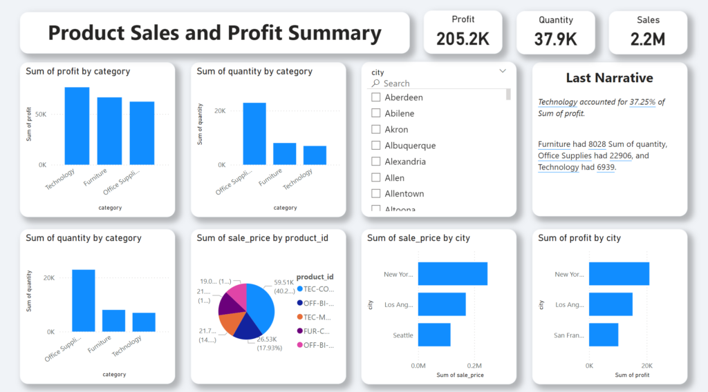
I uploaded this power bi dashboard as pbix file in my github

• Product sales and profit summary
• Regional performance metrics
• Category-wise analysis
• Growth trends

📈 Key Findings

• Technology accounted for 37.25% of total profit
• Furniture had 8,028 units in quantity
• Office Supplies reached 22,906 units
• Technology achieved 6,939 units

🔄 Project Workflow

1. Data Collection → 2. Cleaning → 3. Database Import → 4. Analysis → 5. Visualization

🔄 Project Source code : https://github.com/seotanvirbd/kaggle-python-sql

👨‍💻 Contact Information

• WhatsApp: Contact Me
• Facebook: seotanvirbd
• LinkedIn: seotanvirbd
• YouTube: @tanvirbinali2200
• Email: tanvirafra1@gmail.com
• Blog & Portfolio: seotanvirbd.com
• github : https://github.com/seotanvirbd/